Linear Model Diagnostics (and What to Do if You Flunk One)
The linear model works great until it doesn’t. Alternatively: I accept the model’s output only the extent to which I accept its assumptions and whether the model estimated satisfies those assumptions. There are myriad assumptions in the linear model and we can’t possibly go over them all in the confines of a single lab session in such a hurried course on quantitative methods. We’ll focus on a few key ones here.
Download the R script for this tutorialElsewhere in My R Cinematic Universe
I will be doing a lot of self-plagiarism in this particular script. I taught earlier versions of to MA students in this department, and to PhD students at my previous employer. This version is a bit more streamlined, but the verbosity of previous versions of it might be useful to look over for you.
I’ve also written elsewhere about how cool bootstrapping
is,
and about assorted heteroskedasticity robust standard
errors.
The latter of the two has an IR application you might find interesting.
The former is illustrative of what exactly the procedure is doing and
how you could do it yourself. Finally, IRIII.2 students in our
department also get the same “check this shit out” approach to
{modelsummary}.
You all will be saying hi to my mom in Ohio a lot.
Finally, I want to make sure you all understand what happens in the linear model when there are log-transformed variables on one or both sides of the regression equation. A shorthand way of thinking about this is that log transformations proportionalize (sic) changes on the untransformed scale. Please read that blog post carefully.
If I link it here, it’s because I’m asking you to look at it. Look at it as it might offer greater insight into what I’m doing and what I’m trying to tell you.
R Packages/Data for This Session
You should’ve already installed the R packages for this lab session.
{tidyverse} will be for all things workflow. {stevedata} will have
data sets and {stevemisc} has some assorted helper functions.
{lmtest} has some formal diagnostic tests and convenience functions
for summarizing standard error adjustments done by the {sandwich}
package. {modelsummary} is awesome and you’ll kind of see what it’s
doing along the way. {stevethemes} is optional, but I want to use it.
I’ll offer a nod to the {car} package that is optional, but has a
function that does what linloess_plot() does (but better).
library(tidyverse)
#> ── Attaching core tidyverse packages ──────────────────────── tidyverse 2.0.0 ──
#> ✔ dplyr     1.1.4     ✔ readr     2.1.4
#> ✔ forcats   1.0.1     ✔ stringr   1.5.0
#> ✔ ggplot2   4.0.0     ✔ tibble    3.2.1
#> ✔ lubridate 1.9.2     ✔ tidyr     1.3.0
#> ✔ purrr     1.1.0
#> ── Conflicts ────────────────────────────────────────── tidyverse_conflicts() ──
#> ✖ dplyr::filter() masks stats::filter()
#> ✖ dplyr::lag()    masks stats::lag()
#> ℹ Use the conflicted package (<http://conflicted.r-lib.org/>) to force all conflicts to become errors
library(stevedata)
library(stevemisc)
#>
#> Attaching package: 'stevemisc'
#>
#> The following object is masked from 'package:lubridate':
#>
#>     dst
#>
#> The following object is masked from 'package:dplyr':
#>
#>     tbl_df
library(stevethemes) # optional, but I want it...
library(lmtest)
#> Loading required package: zoo
#>
#> Attaching package: 'zoo'
#>
#> The following objects are masked from 'package:base':
#>
#>     as.Date, as.Date.numeric
library(sandwich)
library(modelsummary)
options("modelsummary_factory_default" = "kableExtra")
# ^ this is new. Default is now "tinytable", but much of my code is written
# around `{kableExtra}`. As you develop your skills, you may want to make the
# pivot to `{modelsummary}`'s default.
theme_set(theme_steve()) # optional, but I want it...
I want to add here that the output format of this script, if you’re
reading it on my website, is to Markdown. The tables themselves are
HTML, which Markdown can handle quite nicely through Github. However,
there is a lever I need to toggle to disable the table captions from
also becoming standalone paragraphs in Markdown format. I don’t know
what that lever is based on my cornball workflow spinning this .R file
to a .md file. This is not a problem you will have formatting for
LaTeX or HTML, but it will make for a somewhat clumsy viewing experience
on the course website. Again, you’ll be saying hi to my Mom a lot. She
lives in Ohio.
Okay then, let’s get on with the show.
The Data We’ll Be Using
I’ll be using the states_war data set in {stevedata}. You can find
more information about this data set by typing this into your RStudio
console.
?states_war
The data offer an opportunity to explore the correlates of performance in war in a way inspired by Valentino et al. (2010). The authors primarily focus on democracy and how democracies allegedly minimize the costs of war through assorted means. We’ll do the same here.
Let’s offer a spiritual replication of the second model of Table 1,
focusing on military fatalities (which is the explicit focus of the
Gibler-Miller conflict data we’ll be using). However, we need to create
some variables. First, we’re going to create a kind of “loss exchange
ratio” variable. Formally, this variable is equal to the fatalities
imposed on the enemy combatant(s) divided over the fatalities suffered
by the state, adding 1 to the denominator of that equation to prevent
division by 0. We’ll create this one, and another that’s proportional
(i.e. imposed fatalities over imposed fatalities and state’s own
fatalities). Play with this to your heart’s content.1 Second, we’re
going to create an initiator variable (init) to isolate those states
that make conscious forays into war. From my experience creating data
for {peacesciencer}, it is usually (though not always) the case that
you can discern initiation from whether it’s on the Side A and/or it’s
an original participant. To get to the point, the initiator variable
will be 1 if 1) it’s on Side A (i.e. the side that made the first
incident) and it’s an original participant and 2) if it’s not an
original participant (often meaning it self-selected into the conflict).
Otherwise, it will be a 0.
states_war %>%
  mutate(ler = oppfatalmin/(fatalmin + 1),
         lerprop = oppfatalmin/(fatalmin + oppfatalmin),
         init = case_when(
           sidea == 1 & orig == 1 ~ 1,
           orig == 0 ~ 1,
           TRUE ~ 0
  )) -> Data
Now, let’s do a kind-of replication of the second model in Table 1,
where we’ll model the first loss exchange ratio variable (LER) we
created (ler) as a function of democracy (xm_qudsest), GDP per
capita (wbgdppc2011est), the initiator variable (init), the military
expenditures of the state (milex), the duration of the participant’s
stay in conflict (mindur), and the familiar estimate of power provided
by CoW’s National Material Capabilities data as the composite index of
national capabilities (cinc).
M1 <- lm(ler ~ xm_qudsest + wbgdppc2011est + init + milex + xm_qudsest +
           mindur + cinc,
         Data)
Okie doke, let’s see what we got.
summary(M1)
#>
#> Call:
#> lm(formula = ler ~ xm_qudsest + wbgdppc2011est + init + milex +
#>     xm_qudsest + mindur + cinc, data = Data)
#>
#> Residuals:
#>      Min       1Q   Median       3Q      Max
#> -1710.43    -4.76     4.30    15.07  2231.12
#>
#> Coefficients:
#>                  Estimate Std. Error t value Pr(>|t|)
#> (Intercept)     3.117e+01  6.224e+01   0.501    0.617
#> xm_qudsest      9.453e+00  1.655e+01   0.571    0.568
#> wbgdppc2011est -3.328e+00  7.472e+00  -0.445    0.656
#> init           -8.634e+00  2.762e+01  -0.313    0.755
#> milex           5.969e-06  4.493e-07  13.285   <2e-16 ***
#> mindur         -5.570e-03  2.240e-02  -0.249    0.804
#> cinc           -1.420e+02  2.005e+02  -0.709    0.479
#> ---
#> Signif. codes:  0 '***' 0.001 '**' 0.01 '*' 0.05 '.' 0.1 ' ' 1
#>
#> Residual standard error: 192.4 on 245 degrees of freedom
#>   (32 observations deleted due to missingness)
#> Multiple R-squared:  0.4417, Adjusted R-squared:  0.428
#> F-statistic:  32.3 on 6 and 245 DF,  p-value: < 2.2e-16
I can already anticipate some design decisions got us to this point, but the model suggests only military expenditures matter to understanding performance in war. Higher values of military expenditures coincide with higher LER. That tracks, at least.
Now, let’s do some diagnostic testing.
Linearity
OLS assumes some outcome y is a linear function of some right-hand predictors you include in the model. That is, the estimated value itself follows that linear formula, and the values themselves are “additive” (i.e. y = a + b + c). There are various diagnostic tests for the linearity assumption, including some outright statistical tests that are either not very good at what they purport to do (Rainbow test), or awkwardly implemented (Harvey-Collier test).
This is why I encourage you to explore this visually. For one, start with arguably the most useful OLS diagnostic plot: the fitted-residual plot. Grab the fitted values from the model and the residuals and create a scatterplot from them. Then, overlay a LOESS smoother over it to check for any irregularities. By definition, the “rise over run” line is flat at 0. The LOESS smoother will communicate whether that’s actually a line of good fit.
Base R has a function that can do this for you. plot() is a default
function in R that, if applied to an object created by lm(), will
create a battery of graphs for you. You just want the first one, which
you can specify with the which argument. Observe.
plot(M1, which=1)
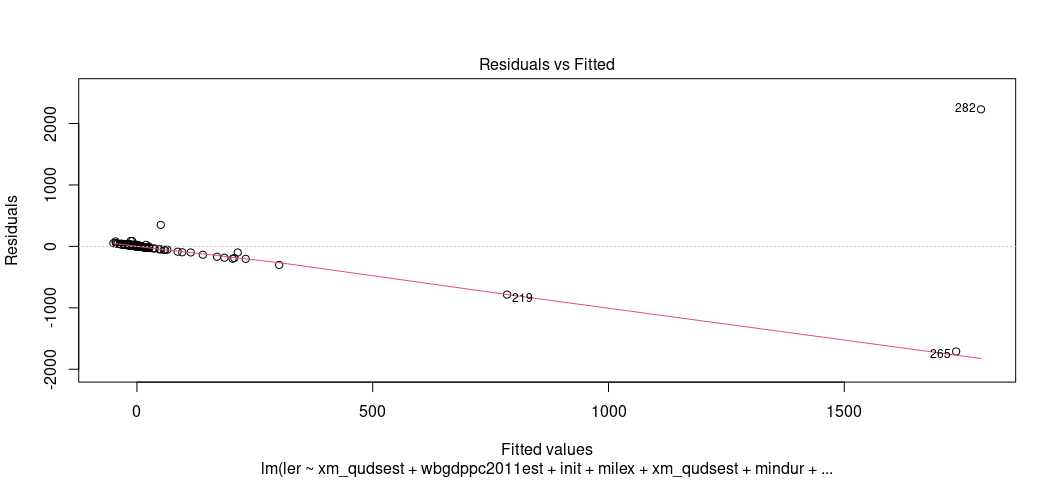
Eww, gross. That shouldn’t look like that. Gross.
You may also want to use this an opportunity to learn about the
augment() function in {broom}. You can use this to extract pertinent
information from the model. First, let’s see what comes out.
broom::augment(M1)
#> # A tibble: 252 × 14
#>    .rownames     ler xm_qudsest wbgdppc2011est  init milex mindur    cinc
#>    <chr>       <dbl>      <dbl>          <dbl> <dbl> <dbl>  <dbl>   <dbl>
#>  1 1          0.0270   -1.58              7.36     0   672    259 0.00559
#>  2 2         35.7       0.376             8.42     1 36520    259 0.298
#>  3 3          0.933    -1.58              1.55     1   211    122 0.00353
#>  4 5          0.593    -1.58              7.93     1  1270    527 0.0114
#>  5 6          1.57     -1.05              6.54     0  6278    527 0.0714
#>  6 9         76        -0.0626            8.22     1 16462    257 0.0441
#>  7 10        78         0.00633           8.15     1 12506    257 0.0289
#>  8 11        15.9       0.226             8.63     1 37508    257 0.127
#>  9 12         2.09      0.981             8.88     1 38588    257 0.185
#> 10 13         7.56      0.737             8.98     1 63547    257 0.169
#> # ℹ 242 more rows
#> # ℹ 6 more variables: .fitted <dbl>, .resid <dbl>, .hat <dbl>, .sigma <dbl>,
#> #   .cooksd <dbl>, .std.resid <dbl>
# ?augment.lm() # for more information
We want just the fitted values and the residuals here. The former goes on the x-axis and the latter goes on the y-axis for the plot to follow.
broom::augment(M1) %>%
  ggplot(.,aes(.fitted, .resid)) +
  geom_point(pch = 21) +
  geom_hline(yintercept = 0, linetype="dashed", color="red") +
  geom_smooth(method = "loess")
#> `geom_smooth()` using formula = 'y ~ x'
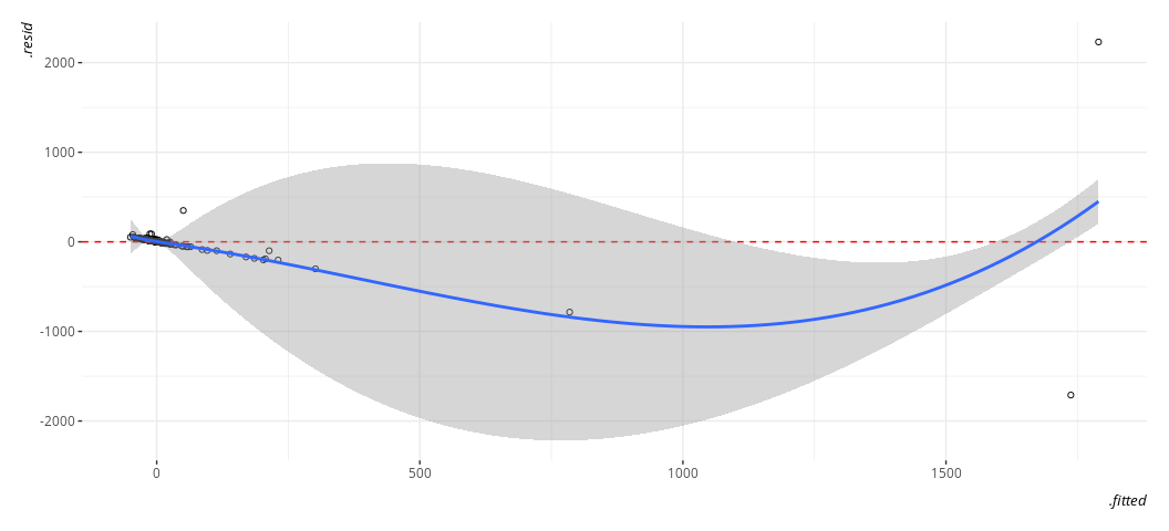
Again, gross. Just, eww. Gross.
You should’ve anticipated this in advance if you had some subject domain expertise. These are large nominal numbers, in war, that could be decidedly lopsided. For example, here’s the U.S. performance against Iraq in the Gulf War.
Data %>% filter(ccode == 2 & micnum == 3957) %>%
  select(micnum:enddate, fatalmin, oppfatalmin, ler)
#> # A tibble: 1 × 7
#>   micnum ccode stdate    enddate  fatalmin oppfatalmin   ler
#>    <dbl> <dbl> <chr>     <chr>       <dbl>       <dbl> <dbl>
#> 1   3957     2 7/24/1990 1/2/1992      153        4137  26.9
In other words, the U.S. killed almost 27 Iraqi troops for every American soldier killed by the Iraqi military. That’s great for battlefield performance from the perspective of the Department of Defense, but it’s going to point to some data issues for the analyst.
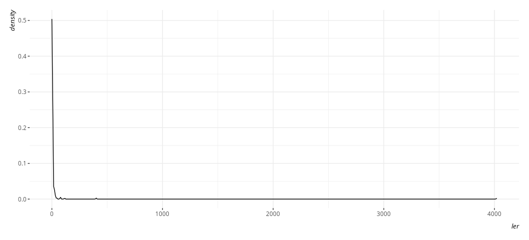
Indeed, here’s what the dependent variable looks like.
Data %>%
  ggplot(.,aes(ler)) +
  geom_density()
Here, btw, is what it’s natural logarithm would look like, and what the proportion variable we created would look like by way of comparison. Believe me when I say I know what I’m doing with the code here. Trust me; I’m a doctor.
Data %>%
  select(ler, lerprop) %>%
  mutate(log_ler = log(ler + 1)) %>%
  gather(var, val) %>%
  ggplot(.,aes(val)) +
  geom_density() +
  facet_wrap(~var, scales='free', nrow= 3)
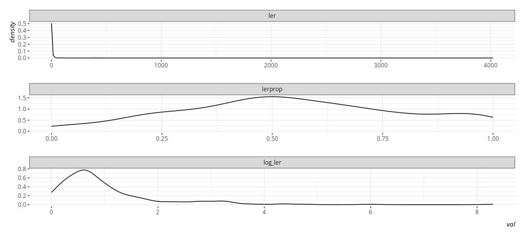
The linear model does not require normally distributed DVs in order to
extract (reasonably) linear relationships. However, we should’ve not
done this, and we should’ve known in advance that we should not have
done this. What estimate of central tendency could we expect from a
variable that looks like this? So, let’s take a step back and
re-estimate the model two ways. The first will do a +1 and log of the DV
and the second will use the proportion variable we created earlier. This
might be a good time as well to flex with the update() function in R.
Data %>% mutate(ln_ler = log(ler + 1)) -> Data

M2 <- update(M1, ln_ler ~ .)
M3 <- update(M1, lerprop ~ .)
Briefly: this is just updating M1 to change the two DVs. A dot (.)
is a kind of placeholder in R to keep “as is.” You can read ~ . as
saying “regressed on the same stuff as before and keeping the other
arguments we supplied to it before (like the data).” You’ll see me
return to more uses of this with the wls() function, which really
wants a data set with no missing values or for you to have supplied
na.action=na.exclude as an optional argument in the lm() function.
We’ll deal with this detail later.
Now, let’s also flex our muscles with modelsummary() to see what these
alternate estimations mean for the inferences we’d like to report.
modelsummary(list("LER" = M1,
                  "log(LER + 1)" = M2,
                  "LER Prop." = M3),
             title = "Hi Mom!",
             stars = TRUE,
             )
| LER | log(LER + 1) | LER Prop. | |
|---|---|---|---|
| (Intercept) | 31.170 | 0.352 | 0.364*** |
| (62.237) | (0.302) | (0.076) | |
| xm_qudsest | 9.453 | 0.245** | 0.075*** |
| (16.547) | (0.080) | (0.020) | |
| wbgdppc2011est | -3.328 | 0.083* | 0.022* |
| (7.472) | (0.036) | (0.009) | |
| init | -8.634 | 0.120 | 0.050 |
| (27.620) | (0.134) | (0.034) | |
| milex | 0.000*** | 0.000*** | 0.000 |
| (0.000) | (0.000) | (0.000) | |
| mindur | -0.006 | -0.000+ | -0.000 |
| (0.022) | (0.000) | (0.000) | |
| cinc | -142.038 | 0.722 | 0.233 |
| (200.469) | (0.972) | (0.245) | |
| Num.Obs. | 252 | 252 | 246 |
| R2 | 0.442 | 0.239 | 0.160 |
| R2 Adj. | 0.428 | 0.220 | 0.139 |
| AIC | 3374.9 | 689.1 | -7.8 |
| BIC | 3403.1 | 717.3 | 20.2 |
| Log.Lik. | -1679.454 | -336.530 | 11.907 |
| RMSE | 189.72 | 0.92 | 0.23 |
|
|||
The results here show that it’s not just a simple matter that “different DVs = different results”. Far from it. Different reasoned design decisions can be the matter of the different results you observe. Using more reasonable estimates of battlefield performance (either logged loss exchange ratio or its proportion form) results in models that make more sense with respect to the underlying phenomenon you should care to estimate. In our case, it’s the difference of saying whether there is an effect to note for democracy, GDP per capita, and duration in conflict.
Still, we may want to unpack these models a bit more, much like we did
above. Let’s focus on M2 for pedagogy’s sake, even though there is
more reason to believe the third model is the less offensive of the
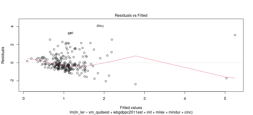
two.2 Let’s get our fitted-residual plot.
broom::augment(M2) %>%
  ggplot(.,aes(.fitted, .resid)) +
  geom_point(pch = 21) +
  geom_hline(yintercept = 0, linetype="dashed", color="red") +
  geom_smooth(method = "loess")
#> `geom_smooth()` using formula = 'y ~ x'
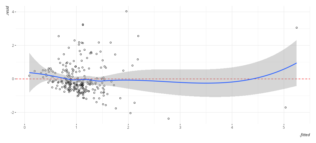
It’s still not ideal. The fitted-residual plot is broadly useful for other things too, and it’s screaming out loud that I have a heteroskedasticity problem and some discrete clusters in the DV. However, it wants to imply some non-linearity as well.
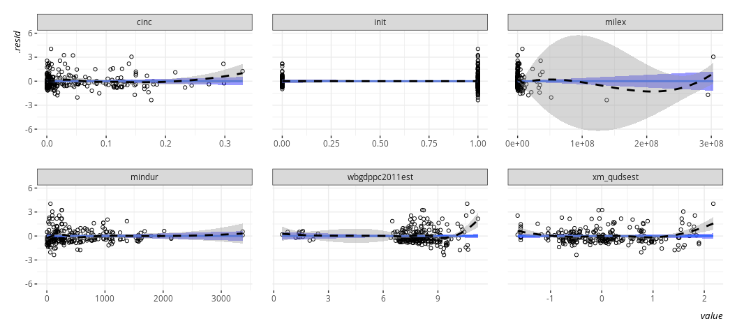
One limitation of the fitted-residual plot, however, is that it won’t
tell you where exactly the issue might be. That’s why I wrote the
linloess_plot() in {stevemisc}. This plot takes a model object and,
for each right-hand side variable, draws a rise-over-run line of best
fit and the LOESS smoother. Do note this tells you nothing about binary
IVs, but binary IVs aren’t the problem here.
linloess_plot(M2, pch=21)
#> `geom_smooth()` using formula = 'y ~ x'
#> `geom_smooth()` using formula = 'y ~ x'
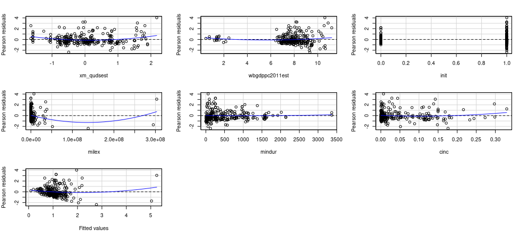
{car} has this one for you, if you’d like. I’ll concede it works
better than my function at the moment.
car::residualPlots(M2)
#>                Test stat Pr(>|Test stat|)
#> xm_qudsest        3.3532        0.0009258 ***
#> wbgdppc2011est    1.7566        0.0802457 .
#> init              0.1241        0.9013501
#> milex             2.7593        0.0062310 **
#> mindur            0.3153        0.7527727
#> cinc              1.3051        0.1931042
#> Tukey test        4.7625        1.912e-06 ***
#> ---
#> Signif. codes:  0 '***' 0.001 '**' 0.01 '*' 0.05 '.' 0.1 ' ' 1
The thing I like about this kind of plot is that it can point to multiple problems, though it won’t point you in the direction of any potential interactions. No matter, here it points to several things that I may want to ask myself about the data. I’ll go in order I see them.
-
Does democracy need a square term? It seems like the most autocratic and the most democratic perform better than those democracies “in the middle”. There’s ample intuition behind this in the democratic peace literature, which emphasizes there is a real difference between a democracy like Sweden and a fledgling democratizing state like mid-1990s Serbia. Intuitively, there is also a qualitative difference between a durable autocracy like Iran now versus a fledgling autocracy like Iran in the early 1980s. We might be seeing that here.
-
The GDP per capita variable has some clusters. It’s already log-transformed, so I’m disinclined to take a log of a log. It’s technically benchmarked in 2011 USD, so there’s not an issue of nominal or real dollars here. Some states are just poor? In our data, I see a jump from 2.428 (Mecklenburg in the First Schleswig War) to 5.815 (i.e. Ethiopia in the Second Italian-Ethiopian War). A few things might be happening here, and it’s worth noting estimates of GDP per capita in the 19th century are always tentative and prone to some kind of measurement error. It might be ideal to proportionalize (sic) these, much like we did with the LER variable. However, that would require more information (on my end, behind the scenes) than we have here. Perhaps we just make a poverty dummy here and leave well enough alone, mostly to see if there is any sensitivity to those observations. The line doesn’t look like it’s affected.
-
It might make sense to log-transform military expenditures and duration. We’d have to do a +1-and-log to expenditures because there are states in war that don’t register in the thousands, per the National Material Capabilities data.
With that out of the way, let’s create some variables of interest to us and re-estimate Model 2.
Data %>%
  mutate(povdum = ifelse(wbgdppc2011est < 4, 1, 0),
         ln_mindur = log(mindur),
         ln_milex = log(milex + 1)) -> Data


M4 <- lm(ln_ler ~ xm_qudsest + I(xm_qudsest^2) +
           wbgdppc2011est + ln_milex + ln_mindur + cinc,
         Data)
summary(M4)
#>
#> Call:
#> lm(formula = ln_ler ~ xm_qudsest + I(xm_qudsest^2) + wbgdppc2011est +
#>     ln_milex + ln_mindur + cinc, data = Data)
#>
#> Residuals:
#>     Min      1Q  Median      3Q     Max
#> -1.8790 -0.5625 -0.1934  0.3217  5.8821
#>
#> Coefficients:
#>                  Estimate Std. Error t value Pr(>|t|)
#> (Intercept)      0.550520   0.383058   1.437  0.15194
#> xm_qudsest       0.253293   0.081828   3.095  0.00219 **
#> I(xm_qudsest^2)  0.284855   0.071087   4.007 8.16e-05 ***
#> wbgdppc2011est   0.076564   0.042133   1.817  0.07040 .
#> ln_milex        -0.007327   0.021925  -0.334  0.73854
#> ln_mindur       -0.047257   0.045252  -1.044  0.29737
#> cinc             1.874209   1.015472   1.846  0.06615 .
#> ---
#> Signif. codes:  0 '***' 0.001 '**' 0.01 '*' 0.05 '.' 0.1 ' ' 1
#>
#> Residual standard error: 0.9609 on 245 degrees of freedom
#>   (32 observations deleted due to missingness)
#> Multiple R-squared:  0.1928, Adjusted R-squared:  0.173
#> F-statistic: 9.753 on 6 and 245 DF,  p-value: 1.232e-09
I don’t think it’s going to be an issue, but now I’m curious…
summary(update(M4, . ~ . -I(xm_qudsest^2), data=subset(Data, povdum == 1)))
#>
#> Call:
#> lm(formula = ln_ler ~ xm_qudsest + wbgdppc2011est + ln_milex +
#>     ln_mindur + cinc, data = subset(Data, povdum == 1))
#>
#> Residuals:
#>      Min       1Q   Median       3Q      Max
#> -0.30447 -0.12641 -0.03361  0.11062  0.34382
#>
#> Coefficients:
#>                Estimate Std. Error t value Pr(>|t|)
#> (Intercept)     -3.7055     1.9102  -1.940   0.0843 .
#> xm_qudsest      -0.3168     0.1770  -1.789   0.1072
#> wbgdppc2011est   0.3990     0.3716   1.074   0.3109
#> ln_milex         0.5037     0.2388   2.109   0.0642 .
#> ln_mindur        0.1930     0.1080   1.787   0.1076
#> cinc           -70.9074    26.3614  -2.690   0.0248 *
#> ---
#> Signif. codes:  0 '***' 0.001 '**' 0.01 '*' 0.05 '.' 0.1 ' ' 1
#>
#> Residual standard error: 0.2332 on 9 degrees of freedom
#>   (3 observations deleted due to missingness)
#> Multiple R-squared:  0.628,  Adjusted R-squared:  0.4213
#> F-statistic: 3.038 on 5 and 9 DF,  p-value: 0.07031
# ^ you can read this `update()` as "update M4, keep DV and bulk of IVs, but
#   remove the square term and change the data to just those in Data where
#   povdum == 1.
We don’t have a lot of observations to play with here, and the observations affected here are decidedly unrepresentative of the overall population of cases. I wouldn’t sweat this issue, other than perhaps as a call to restrict any serious analysis to just the 20th century when we developed better capacity for calculating estimates of economic size and wealth. All the observations affected here are in the 19th century and, wouldn’t you know it, all concern the wars of Italian/German unification.
You’re welcome to play more with the diagnostics of these models, though it comes with the caveat that you’re making linear assumptions anyway when you estimate this model. Don’t go chasing waterfalls, only the rivers and the lakes to which you are used… to. I know you’re going to have it your way or (more than likely) use no statistical model at all. Let’s just not move too fast.3
Independence
The linear model assumes the independence of the model’s errors and that any pair of errors are going to be uncorrelated with each other. Past observations (and past errors) should not inform other pairs of errors. In formal terms, this assumption seems kind of Greek to students. In practice, think of it this way. A lot of the theoretical intuition behind OLS is assuming something akin to a simple random sample of the population. You learned central limit theorem by this point and how you can simulate that. However, you may have a data set that does not look like this.
In other words, this assumption is going to be violated like mad in any design that has a time-series, spatial, or multilevel component. For students new to this stuff, you should be able to anticipate ahead of time when your errors are no longer independent of each other.
The implications of non-independent errors—aka “serial correlation” or “autocorrelation”—are generally more about the variance of the estimator than the estimator itself. That said, there is reason to believe the standard errors are wrong and this can have important implications for statistical inference you’d like to do. No matter, this is a huge assumption about OLS and violating it ultimately means OLS loses its inferential value. The data are no longer randomly sampled in that sense.
Once you know under what conditions that autocorrelation is going to happen, you can probably skip this and go right to assorted tricks that you know will work given the nature of your serial correlation. So, this is going to be a curious exercise I’m going to have you do here. The fundamental grouping effect here is primarily “spatial” or cross-sectional (in that it deals with state groupings) but the primary tests we teach around this particular assumption are temporal (i.e. we’re going to prime you in the advanced level to think about time series and panel models). I just want to reiterate this is something you should really know in advance about your data, and should assume a priori about your data. The primary tests of interest are always geared toward temporal attributes of a data set (which, again, you should know in advance).
Anywho, if you have a random walk time series, you know those can typically be first-differenced in order to strip out the source of autocorrelation. If you have some type of “spatial” serial correlation (e.g. citizens nested in countries, students nested in schools), you can employ some kind of fixed effects or random effects to outright model the source of unit heterogeneity. No matter, the “textbook” tests for these are typically in the time series case and involve the Durbin-Watson test or the Breusch-Godfrey test.
Of the two, practitioners I’ve read seem to favor the latter over the
former. The Durbin-Watson test has some pretty strong assumptions and
only looks for a order-1 autocorrelation. No matter, it has some
informational value when you get deeper into the weeks of time series
stuff. Both can be estimated by way of the {lmtest} package. Let’s go
back to our model and apply both.
dwtest(M2)
#>
#>  Durbin-Watson test
#>
#> data:  M2
#> DW = 1.7386, p-value = 0.01523
#> alternative hypothesis: true autocorrelation is greater than 0
bgtest(M2)
#>
#>  Breusch-Godfrey test for serial correlation of order up to 1
#>
#> data:  M2
#> LM test = 2.3983, df = 1, p-value = 0.1215
The “null” hypothesis of both tests is “no autocorrelation.” The alternative hypothesis is “autocorrelation.” When the p-value is sufficiently small, it indicates a problem. Here, they seem to suggest some kind of autocorrelation, though the data aren’t exactly a panel or a time series. Understand, again, these tests are making particular assumptions about your data that we don’t quite have, and that you should learn to anticipate these issues without needing a textbook test to do it for you. I don’t have the time or opportunity to belabor these issues in detail, but:
-
When you read quant stuff in IR, especially the kind of stuff you might see my name attached to or people I otherwise know, you’ll see so-called “clustered” standard errors that are often “spatial” or cross-sectional in scope. For example, there is good reason to believe the American observations in this model are related to each other. British observations should be related to other British observations, and so on.
-
Much like you’d see in a panel model, you might also see so-called “fixed effects” applied here. This might take on multiple forms. If I had any reason to believe whatsoever that conflicts within particular regions are different from each other, I could create a series of dummies that say “is this war in Europe or not” or “is this in Sub-Saharan Africa or not?” Or, perhaps, I have reason to believe there is a clustering of observation by era or moment in time. The world war eras are different from the Cold War eras, and so on.
I can create these ad hoc with the information available in the data I
have. The stdate column has the start of the first event by the
participant in war. I can extract that with str_sub() (getting the
last four digits), and convert that to a numeric integer for year. Then,
I can use a case_when() call to categorize whether the observation was
before World War I, between and involving both world wars, during the
Cold War, or after the Cold War.
Data %>%
  mutate(year = str_sub(stdate, -4, -1)) %>%
  mutate(year = as.numeric(year)) %>%
  mutate(period = case_when(
    year <= 1913 ~ "Pre-WW1",
    between(year, 1914, 1945) ~ "WW1 and WW2 Era",
    between(year, 1946, 1990) ~ "Cold War",
    year >= 1991 ~ "Post-Cold War"
  )) %>%
  mutate(period = fct_relevel(period, "Pre-WW1", "WW1 and WW2 Era",
                              "Cold War")) -> Data

M5 <- update(M2, . ~ . + period, Data)
modelsummary(list("log(LER + 1)" = M2,
                  "w/ Period FE" = M5),
             stars = TRUE,
             title = "Hi Mom!",
)
| log(LER + 1) | w/ Period FE | |
|---|---|---|
| (Intercept) | 0.352 | 0.321 |
| (0.302) | (0.298) | |
| xm_qudsest | 0.245** | 0.251** |
| (0.080) | (0.080) | |
| wbgdppc2011est | 0.083* | 0.109** |
| (0.036) | (0.038) | |
| init | 0.120 | 0.130 |
| (0.134) | (0.132) | |
| milex | 0.000*** | 0.000*** |
| (0.000) | (0.000) | |
| mindur | -0.000+ | -0.000 |
| (0.000) | (0.000) | |
| cinc | 0.722 | 0.761 |
| (0.972) | (1.033) | |
| periodWW1 and WW2 Era | -0.526** | |
| (0.165) | ||
| periodCold War | -0.300+ | |
| (0.165) | ||
| periodPost-Cold War | -0.070 | |
| (0.232) | ||
| Num.Obs. | 252 | 252 |
| R2 | 0.239 | 0.274 |
| R2 Adj. | 0.220 | 0.247 |
| AIC | 689.1 | 683.3 |
| BIC | 717.3 | 722.2 |
| Log.Lik. | -336.530 | -330.669 |
| RMSE | 0.92 | 0.90 |
|
||
Do note fixed effects in this application have a tendency to “demean” other things in the model, and they have a slightly different interpretation. For example, though both are “significant” and “look the same”, the GDP per capita effect is now understood as the effect of increasing GDP per capita within periods rather than higher levels of GDP per capita, per se. You do observe some period weirdness. Compared to the pre-WWI era, logged LER is generally lower in the interwar years and generally lower in the Cold War, importantly partialing out the other information in the model. No matter, if you have autocorrelation, you have to tackle it outright or your OLS model has no inferential value. The exact fix depends on the exact nature of the problem, which will definitely depend on you knowing your data well and what you’re trying to accomplish.
Normality (of the Errors)
OLS assumes the errors are normally distributed. This is often conflated with an assumption that the outcome variable is normally distributed. That’s not quite what it is. It does imply that the conditional distribution of the dependent variable is normal but that is not equivalent to assuming the marginal distribution of the dependent variable is normal. At the end of the day, the assumption of normality is more about the errors than the dependent variable even as the assumption about the former does strongly imply an assumption about the latter.
Violating the assumption of a normal distribution of the errors is not as severe as a violation of some of the other assumptions. The normality assumption is not necessary for point estimates to be unbiased. In one prominent textbook on statistical methods, Gelman and Hill (2007, p. 46) say the normality assumption is not important at all because it has no strong implication for the regression line. I think this follows because Gelman and Hill (2007)—later Gelman, Hill, and Vehtari (2020)—are nowhere near as interested in null hypothesis testing as your typical social scientist likely is. No matter, violating the assumption of a normal distribution of errors has some implication for drawing a line that reasonably approximates individual data points (if not the line itself, per se). Thus, you may want to check it, certainly if you have a small data set.
My misgiving with these normality tests is that they all suck, even at
what they’re supposed to do. The “textbook” normality tests involve
extracting the residuals from the model and checking if their
distribution is consistent with data that could be generated by a normal
distribution. The two implementations here are typically base R. One is
the Shapiro-Wilk test. The other is the Kolmogorv-Smirnov test. There
are more—like the Anderson-Darling test—which you can also do and is
communicating the same thing. You can explore a few of these in the
{nortest} package.
shapiro.test(resid(M2))
#>
#>  Shapiro-Wilk normality test
#>
#> data:  resid(M2)
#> W = 0.90417, p-value = 1.349e-11
ks.test(resid(M2), y=pnorm)
#>
#>  One-sample Kolmogorov-Smirnov test
#>
#> data:  resid(M2)
#> D = 0.14934, p-value = 2.626e-05
#> alternative hypothesis: two-sided
When p-values are sufficiently small, these tests are saying “I can determine these weren’t generated by some kind of normal distribution.” My misgiving with these particular tests are multiple. One, you can dupe them pretty easily with a related distribution that looks like it, but is not it (e.g. Student’s t). For example, let me cheese the Shapiro test with the Poisson distribution.
set.seed(8675309)
shapiro.test(lambdas <- rpois(1000, 100))
#>
#>  Shapiro-Wilk normality test
#>
#> data:  lambdas <- rpois(1000, 100)
#> W = 0.99791, p-value = 0.2457
# c.f. http://svmiller.com/blog/2023/12/count-models-poisson-negative-binomial/
I should not have passed this test, and yet I did. These aren’t normally distributed. They’re Poisson-distributed, and can’t be reals. Second, these normality tests are deceptively just a test of sample size. The more observations you have, the more sensitive the test is to any observation in the distribution that looks anomalous. Three, textbooks typically say to use the K-S test if you have a large enough sample size, but, from my experience, that’s the test that’s most easily duped.
Here’s what I recommend instead, knowing that the normality assumption of errors is one of the least important assumptions: visualize this instead. For one, the “textbook” visual diagnostic is the Q-Q plot. This is actually a default plot in base R for linear models if you know where to look.
plot(M2, which=2)
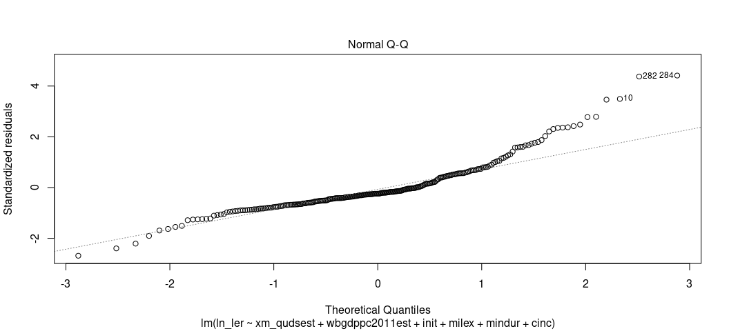
The Q-Q plots the theoretical quantiles of the residuals against the standardized residuals. Ideally, they all fall on a nice line. Here, they don’t, suggesting a problem. The negative residuals are more negative than expected at the tail end of the distribution (which is almost always unavoidable for real-world data at the tails) but the higher residuals are more positive than expect for the higher quantiles. This one is more problematic. You could’ve anticipated this knowing that there is still a right skew in the DV even after its logarithmic transformation.
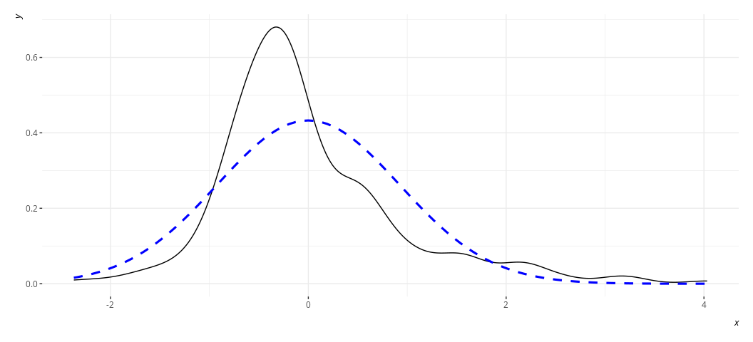
I mentioned in lecture that a better way of gauging just how severe the
issue is will involve generating a density plot of the residuals against
a stylized density plot matching the description of the residuals
(i.e. with a mean of 0 and a standard deviation equal to the standard
deviation of the residuals). It would look something like this for M2.
rd_plot(M2)
Or this for M3:
rd_plot(M3)
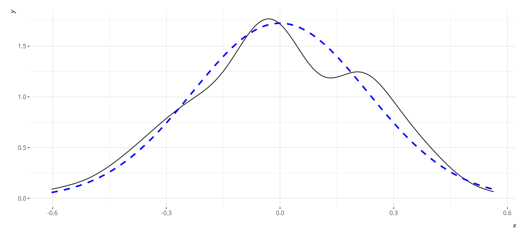
In these plots, the black solid line is a density plot of the actual
residuals whereas the blue, dashed line is a density plot of a normal
distribution with a mean of 0 and a standard deviation equal to the
standard deviation of the residuals. The real thing will always be kind
of lumpy in some ways when you’re using actual data. Ask yourself how
bad it is. I’d argue that the distribution is not acceptable in the case
of M2, though reasonably approximated in M3. Both results are fairly
similar to each other in the stuff we care about.
Your solution to this particular “problem” will depend on what exactly you’re doing in the first place. The instances in which these plots look really problematic will be situations like these. Your model may have relatively few covariates and the covariates you do include are dummy variables. If you have so few observations in the model (i.e. I can count the number of observations in the model on one or three hands), any distribution of residuals will look crazy. That’s probably not your case, especially as you’ve thought through the data-generating process for your dependent variable. It’s more likely the case that you have a discrete dependent variable and you’re trying to impose a linear model on it. The end result is a subset of residuals that look kind of wonky at the tails of the distribution. Under those conditions, it makes more sense to use the right model for the nature of your dependent variable. If your DV is binary, consider a logistic regression. If you’re trying to model variation in a 5-item Likert measure, consider the ordinal logistic regression. If you have a proportion with observations appearing at the exact limit of the proportion, consider some kind of beta regression. Are you trying to model a “count” variable (i.e. an integer), especially one that has some kind of skew? Maybe you want a Poisson regression, or negative binomial.
Either way, the solution to the non-normality of the residuals involves outright modeling the kind of data that presents this kind of non-normality. The assumption, to be clear, is about the errors, but the “problem” and the “solution” often point to what exactly your dependent variable looks like and whether OLS is the right model for the job.
Equal Error Variance (Homoskedasticity)
The final diagnostic test you should run on the OLS model involves assessing whether the distribution of residuals is constant across the range of the model. OLS assumes that the variance of the errors is the same regardless of the particular value of x. This is often called “homoskedasticity”, mostly in juxtaposition to the violation of this assumption: “heteroskedasticity.” The change of prefix should be clear to what is implied here. Heteroskedasticity often means the errors are typically a function of something else in the model.
The implications for violating the assumption of homoskedasticity are
more nuisance than real problem. Unequal/non-constant variance does not
affect the XB part of the regression model, but it does have
implications for predicting individual data points. Here, the
implication is similar to the implication of violating the assumption of
normally distributed errors. However, it’s more severe than the
non-normality of residuals. If null hypothesis significance testing is
part of your research design (and it is), heteroskedasticity means the
standard errors of your estimates are wrong. Worse yet: they’ll be wrong
in ways you don’t know until you start digging further into what your
data and model look like.
There are two ways to assess whether you have a heteroskedasticity problem in your OLS model. The first is the fitted-residual plot. You can ask for that again. This time, have your eye draw kind of an upper bound and lower bound on the y-axis (for the residuals). Are those lines flat/pattern-less? Tell-tale cases of heteroskedasticity like we discussed in lecture are cases where you have a cone pattern emerge. Sometimes it’s not as obviously cone-shaped. This one is 100% cone-shaped.
plot(M2, which=1)
I think I see a pattern, and certainly the pattern of residuals don’t
look like random buckshot like I’d want. Fortunately, there’s an actual
test you can use that’s available in the {lmtest} package. It’s the
Breusch-Pagan test. The null hypothesis of the test is homoskedasticity.
The alternate hypothesis is heteroskedasticity. If the p-value is
sufficiently small, you have a problem.
bptest(M2)
#>
#>  studentized Breusch-Pagan test
#>
#> data:  M2
#> BP = 49.163, df = 6, p-value = 6.918e-09
Looks like we have a problem, but what’s the solution? Unfortunately, there’s no quick fix, per se, because any single solution to heteroskedasticity depends on the exact nature of heteroskedasticity and whether you know for sure that’s the case. If you have positive reals on either side of the regression equation, and there’s some kind of positive skew that’s causing residuals to fan out, you can consider some kind of logarithmic transformation to impose normality on the variable(s). Is it an outlier/influence observation that’s causing this? If so, consider punting out the observation from the model. At least, consider it. I’ll note that outliers/influence are not sufficient justification to exclude an observation from a regression model. You should only do that if it’s unrepresentative of the underlying population, not necessarily because it’s anomalous in the underlying population.
Therefore, “solutions” to heteroskedasticity are often just alternative specifications of the model and seeing if the core results from the base model change in any meaningful way. There are a few paths you may want to explore.
The basic “textbook” approach is weighted least squares. I mentioned in
lecture that this approach is kind of convoluted. It’s not complicated.
It’s just convoluted. The procedure here starts with running the
offending model (which we already did; it’s M2). Then, grab the
residuals and fitted values from the model. Next, regress the absolute
value of the residuals on the fitted values of the original model.
Afterward, extract those fitted values, square them and divide 1 over
those values. Finally, apply those as weights in the linear model once
more for a re-estimation.
An older version of this script showed you how you can do it yourself.
Just have {stevemisc} do it for you with the wls() function. Just be
mindful that the wls() function isn’t keen on data frames where
observations have NAs. If you have those, and just want to ignore it and
proceed, you may want to include an na.action = na.exclude as an
optional argument in lm(). We can cheese that here with an update().
modelsummary(list("log(LER)" = M2,
                  "WLS" = wls(update(M2, na.action=na.exclude))),
             stars = TRUE,
             title = "Hi Mom!",
             gof_map = c("nobs", "adj.r.squared"))
| log(LER) | WLS | |
|---|---|---|
| (Intercept) | 0.352 | 0.386** |
| (0.302) | (0.139) | |
| xm_qudsest | 0.245** | 0.103 |
| (0.080) | (0.065) | |
| wbgdppc2011est | 0.083* | 0.068*** |
| (0.036) | (0.018) | |
| init | 0.120 | 0.182+ |
| (0.134) | (0.093) | |
| milex | 0.000*** | 0.000 |
| (0.000) | (0.000) | |
| mindur | -0.000+ | -0.000 |
| (0.000) | (0.000) | |
| cinc | 0.722 | 0.883 |
| (0.972) | (0.919) | |
| Num.Obs. | 252 | 252 |
| R2 Adj. | 0.220 | 0.117 |
|
||
Re-estimating the model by way of weighted least squares reveals some interesting changes, leaving open the possibility that any inference we’d like to report for the democracy variable, the initiator variable, the military expenditure variable, and the duration variable are functions of the heteroskedasticity and whether we dealt with it in the “textbook” way.
There is an entire branch of econometrics that deals with what to do about your test statistics if you have this problem, and they all seem to have a unifying aversion to the weighted least squares approach. Their point of contention is typically that if the implications of heteroskedasticity is the line is fine but the standard errors are wrong, then the “fix” offered by a textbook is almost guaranteed to redraw lines. They instead offer a battery of methods to recalibrate standard errors based on information from the variance-covariance matrix to adjust for this. This would make the standard errors “robust.”
I mention above that I have an entire blog post that discusses some of
these things in more detail than I will offer here. It’s a lament that
it’s never just “do this and you’re done” thing; it’s always a “fuck
around and see what you find” thing. However, the “classic” standard
error corrections are so-called “Huber-White” standard errors and are
often known by the acronym “HC0”. The suggested defaults you often see
in software for “robust” standard errors are type “HC3”, based on this
offering from Mackinnon and White
(1985).
I can’t really say this with 100% certainty (because you won’t know
until you can see it for yourself) but it’s often the case that older
analyses that report “robust” standard errors are Huber-White (“HC0”)
standard errors and “heteroskedasticity-robust” standard errors in newer
analyses are HC3 standard errors. That’s at least a heuristic I’ve
picked up from my experience. It’s conceivable that “robust” standard
errors in analyses you see 20 years ago might also be type “HC1”. Your
clue for that would be whether the analysis was conducted (or advertised
that it was done) in Stata. “HC1” was (is?) Stata’s default standard
error correction if you attached , robust at the end of the reg
call.4
There’s another approach, which is 100% I’d do if I were presented the opportunity. I’d bootstrap this motherfucker. You likewise have several options here. I maintain it’s fun/advisable to do the bootstrap yourself rather than have some software bundle do it for you, and I have guides on previous course websites and on my blog that show you how to do this. However, we’ll keep it simple and focus on some convenience functions because they also illustrate the myriad options you have. Let’s focus on just two. The first, the simple bootstrap pioneered by Bradley Efron, resamples with replacement from the data and re-runs the model some number of times. In expectation, the mean coefficients of these re-estimated models converge on what it is in the offending model (which you would know from central limit theorem). However, the standard deviation of the coefficients is your bootstrapped standard error.
If you wanted to do any one of these in isolation, you’d want to
leverage the coeftest() function in {lmtest} with the assorted
mechanisms for futzing with the variance-covariance matrix (or other
parts of the model) in the {sandwich} package. For example, what
follows below is going to do the simple bootstrap 1,000 times on M2.
You can set a reproducible seed with the set.seed() function for max
reproducibility, if you’d like.
# set.seed(8675309)
coeftest(M2, vcov = sandwich::vcovBS(M2, R = 1000))
#>
#> t test of coefficients:
#>
#>                   Estimate  Std. Error t value Pr(>|t|)
#> (Intercept)     3.5205e-01  2.1520e-01  1.6360 0.103131
#> xm_qudsest      2.4458e-01  9.7837e-02  2.4999 0.013078 *
#> wbgdppc2011est  8.3176e-02  3.0731e-02  2.7066 0.007277 **
#> init            1.2043e-01  1.0916e-01  1.1033 0.270971
#> milex           1.1194e-08  7.7107e-09  1.4518 0.147847
#> mindur         -1.8977e-04  8.9418e-05 -2.1223 0.034813 *
#> cinc            7.2242e-01  1.0918e+00  0.6617 0.508815
#> ---
#> Signif. codes:  0 '***' 0.001 '**' 0.01 '*' 0.05 '.' 0.1 ' ' 1
coeftest(M2) # compare to what M2 actually is.
#>
#> t test of coefficients:
#>
#>                   Estimate  Std. Error t value  Pr(>|t|)
#> (Intercept)     3.5205e-01  3.0177e-01  1.1666  0.244487
#> xm_qudsest      2.4458e-01  8.0232e-02  3.0484  0.002553 **
#> wbgdppc2011est  8.3176e-02  3.6230e-02  2.2958  0.022533 *
#> init            1.2043e-01  1.3392e-01  0.8993  0.369378
#> milex           1.1194e-08  2.1784e-09  5.1387 5.652e-07 ***
#> mindur         -1.8977e-04  1.0863e-04 -1.7470  0.081893 .
#> cinc            7.2242e-01  9.7200e-01  0.7432  0.458055
#> ---
#> Signif. codes:  0 '***' 0.001 '**' 0.01 '*' 0.05 '.' 0.1 ' ' 1
Take a moment to appreciate that you just ran 1,000 regressions on a 1,000 data replicates in a matter of seconds. Thirty years ago, that would’ve taken a weekend at a supercomputer at some American university with a billion dollar endowment. Neat, huh?
Anywho, the results of the simple bootstrap suggest a precise effect of military expenditures that would not be discerned in the model with heteroskedastic standard errors. The other significant coefficients are still significant, but less precise.
FYI, {modelsummary} appears to be able to do this as well. In this
function, notice what the vcov argument is doing and the order in
which it is doing it.
modelsummary(list("log(LER)" = M2,
                  "WLS" = wls(update(M2, na.action=na.exclude)),
                  "HC0" = M2,
                  "HC3" = M2,
                  "Bootstrap" = M2),
             vcov = list(vcovHC(M2,type='const'),
                         vcovHC(wls(update(M2, na.action=na.exclude))),
                         vcovHC(M2,type='HC0'),
                         vcovHC(M2, type='HC3'),
                         vcovBS(M2)),
             gof_map = c("nobs", "adj.r.squared"),
             title = "Hi Mom! Last time, I promise.",
             stars = TRUE)
| log(LER) | WLS | HC0 | HC3 | Bootstrap | |
|---|---|---|---|---|---|
| (Intercept) | 0.352 | 0.386** | 0.352+ | 0.352 | 0.352+ |
| (0.302) | (0.131) | (0.207) | (0.221) | (0.205) | |
| xm_qudsest | 0.245** | 0.103 | 0.245* | 0.245* | 0.245** |
| (0.080) | (0.082) | (0.095) | (0.099) | (0.092) | |
| wbgdppc2011est | 0.083* | 0.068*** | 0.083** | 0.083** | 0.083** |
| (0.036) | (0.018) | (0.030) | (0.032) | (0.030) | |
| init | 0.120 | 0.182* | 0.120 | 0.120 | 0.120 |
| (0.134) | (0.090) | (0.110) | (0.114) | (0.112) | |
| milex | 0.000*** | 0.000 | 0.000* | 0.000 | 0.000 |
| (0.000) | (0.000) | (0.000) | (0.000) | (0.000) | |
| mindur | -0.000+ | -0.000+ | -0.000* | -0.000* | -0.000* |
| (0.000) | (0.000) | (0.000) | (0.000) | (0.000) | |
| cinc | 0.722 | 0.883 | 0.722 | 0.722 | 0.722 |
| (0.972) | (1.032) | (1.077) | (1.153) | (1.217) | |
| Num.Obs. | 252 | 252 | 252 | 252 | 252 |
| R2 Adj. | 0.220 | 0.117 | 0.220 | 0.220 | 0.220 |
|
|||||
The summary here suggests that we have heteroskedastic errors, and what we elect to do about it—or even if we elect to do anything about it—have implications for the inferences we’d like to report. No matter, the “solution” to heteroskedastic standard errors are more “solutions”, multiple, and involve doing robustness tests on your original model to see how sensitive the major inferential takeaways are to these alternative estimation procedures.
-
The fatalities offered by Gibler and Miller (2024) have high and low estimates. We’ll focus on just the low estimates here. ↩
-
We are also going to leave aside an important conversation to have about just how advisable a +1-and-log really is for isolating coefficients of interest and whether this should be a linear model at all. The linear model is probably “good enough”, and certainly for this purpose. ↩
-
“Creep” is 100% the best single off that record, but didn’t have the Windows 95-era CGI. You know I’m right. Stay out of my mentions. ↩
-
The distinction among these various standard error corrections depends on the intersection of leverage points and sample size. For larger sample sizes, the distinctions don’t really materialize. For smaller sample sizes without a lot of leverage points, type “HC0” and “HC1” tend to underestimate standard errors. For smaller sample sizes with a lot of leverage points, HC3 tends to perform best while “HC0” and HC1” perform worse. While it tracks that “HC3” standard error corrections may want to overestimate standard errors, econometricians tend to like this under the premise that it makes their standard error corrections “conservative” (i.e. it makes it harder to reject the null hypothesis and better hedges against Type I errors). It’s why the R packages that do these standard error corrections prioritize “HC3” over others. In principle, “HC2” is not as conservative as “HC3” and performs better in smaller samples than “HC0” and “HC1”. However, I cannot earnestly tell you ever seeing such a standard error correction in the wild. Imbens and Kolesar (2016) recommend a modified version of it, though. This topic is admittedly kind of frustrating. So much of what’s “suggested” is often an issue of path dependence and an uncritical use of current practice. In other words: we suggest things as defaults because they are defaults. Do what’s been done before. Just because it’s standard practice doesn’t necessarily make it good practice, though. ↩